Dive into Deep Learning Study Notes

Introduction

Four Main Categories

• Analyze pass data, predict future outcome - speech recognition
• Read the questions in text and answer them based on knowledge trained - NLP
• Identify animals from an given image - computer vision
• Promote potential goods to the customer’s based on pass purchasing experience or searches - recommendation engines

Machine Learning Concept

#concept

Even when we don’t know hot to program a hardware to explicitly do certain actions : a application uses microphone to collect inputs and analyze the voice messages. We, the human brains are nonetheless capable of performing the cognitive feat ourselves

How

#parameters #参数 A way to solve problem using “machine learning” is to define a flexible program whose ==behavior== is determined by a number of ==parameters==.

==parameters== are set by ==analyzing dataset== to determine the best possible ==parameter==values.

Parameter, Model, Learning Alogorithm

You can think of the parameters as knobs that we can turn, manipulating the behavior of the program. Once the parameters are fixed, we call the program a ==model==. The set of all distinct programs (input–output mappings) that we can produce just by manipulating the parameters is called a ==family of models==. And the “meta-program” that uses our dataset to choose the parameters is called a ==learning algorithm==.

The Learning

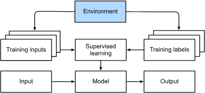
 the learning is the process by which we discover the right setting of the knobs for coercing the desired behavior from our model. In other words, we train our model with data. As shown in Fig. 1.1.2, the training process usually looks like the following:

1. Start off with a randomly initialized model that cannot do anything useful.
2. Grab some of your data (e.g., audio snippets and corresponding {yes,no} labels).
3. Tweak the knobs to make the model perform better as assessed on those examples.
4. Repeat Steps 2 and 3 until the model is awesome.  

Supervised Learning

• Input
• Input label
• predict a designated unknown label based on known inputs given a dataset. #questions
• How should the data be prepared?
• Where to gather all the data?
• How to create the algorithm?

Always

#questions

• Data we can learn from
• Model of how to transform the data
• Objectivefunction that quantified how well the model is doing
• Algorithm to adjust the model’s parameters

What is Data (brief)

• with ==features== that a model can make its prediction on its ==label== (not part of the model’s input - feature)

Fixed-length vector examples

when a example inputs have the same number of numerical features

Variable-length example

• Text
• images with different sizes

  How do we determine/harvest features out of a input?

Training Set vs Testing Set

#objectivefunction

• Objective function - formal measures of how good the model is
• Training Set - A dataset has minimized input error, which will lead to minimized loss function /objective function
• Test Set - held out for evaluation

Models

These models consist of many successive transformations of the data that are chained together top to bottom, thus the name deep learning. On our way to discussing deep models, we will also discuss some more traditional methods. #statisticalmodels

• statistical models can be estimated from data.

Objective Functions

#objectivefunction a mathmatical function to value the how well a model is at its job.

Optimization Algo

an algo that search for the best possble ==parameters for minimizing the loss function/objective function==. Usually based on an popular approach called ==gradient descent==

Kinds of Machine Learning Problems

• Supervised Learning : Feature - label pair, we are the supervisors who provide the model with a dataset consisting of labeled examples.
  • Regression : When labels (e.g., house selling price) are taken on arbitrary numerical values, and we will work on minimizing the squared error
    • How many hours will this surgery take?
    • How much rainfall this town have in the next 6 hours
  • Classification : Identify one* category an example belongs, grouping examples into different categories. Seed for a classifier*.
    • Binary Classification
    • Multiclass Classification
    • Hierarchically structures classes
      • level of classes and sub-classes (dogs, different breeds of dogs)
  • Tagging : Instead of classifying, predict classes that are not mutally exclusive* is called multilabel classification*
  • Search : scoring relevant pages and display them with priorities.
  • Recommendation Systems : Different than ^ is the emphasis on personalization* to specific users.
  • Sequence Learning : Unlike previous model where the test example are forgotten after model processing. This is not ideal for Processing Videos* == Each example (frame) might be drastically different; For more time sensitive problems.
    • Tagging and Parsing : A sequence of aligned text, tagging the word if they are referring entities or direct objects.
    • Automaic Speed Recognition: audio recording
    • Machine Translation: input and output may appear if different order
• Unsupervised and Self-Supervised Learning
  • Clusetering, can we group something together given the
  • Subspace Estimation
  • causality, probabilistic graphical models
• Offline Learning vs Environment aware
  • remember env
  • determine the env
  • shifting dynamics
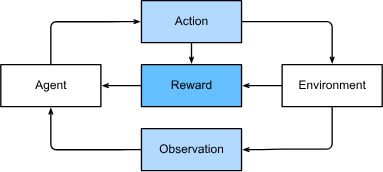
• Reinforcement Learning
  • interacts with env and Take Actions* which actually impacts the environment. (e.g., AlphaGo)
  • Solved the problem where the agent receives observation* from the environment and must chooser an corrsponding action*
  • Goal of the learning is to provide a good mapping from observation of the environment to actions*

Preliminaries

Ndarray

Liner-Algebra

import torch
A = torch.arange(6).reshape(3, 2)
B = A.clone()  # Assign a copy of A to B by allocating new memory

Products

#dot-products
torch.sum(x * y)

#matrix-vector product
A.shape, x.shape, torch.mv(A, x), A@x
#matrix-matrix
B = torch.ones(3, 4)
torch.mm(A, B), A@B

Norms

Measures how big/long a vector/matrix is.

Euclidean norm (l2 norm)

\(\|\mathbf{x}\|_2 = \sqrt{\sum_{i=1}^n x_i^2}.\)

Manhattan distance

\[\|\mathbf{x}\|_1 = \sum_{i=1}^n \left|x_i \right|.\]

Frobenius norm

\(\|\mathbf{X}\|_\textrm{F} = \sqrt{\sum_{i=1}^m \sum_{j=1}^n x_{ij}^2}.\)

Tensor

• Tensor in PyTorch and TensorFlow
• ndarray in MXNet
• NumPy’s ndarray  First, the tensor class supports automatic differentiation. Second, it leverages GPUs to accelerate numerical computation, whereas NumPy only runs on CPUs.

Tensor Operations

x = torch.arange(12, dtype=torch.float32)
x.numel()
12
## Access Shape of the tenso
x.shape

## Reshape the vector into a matrice
x_reshaped=x.reshape(3,4)
tensor([[ 0.,  1.,  2.,  3.],
        [ 4.,  5.,  6.,  7.],
        [ 8.,  9., 10., 11.]])
torch.zeros((2,3,4))

torch.tensor([[2, 1, 4, 3], [1, 2, 3, 4], [4, 3, 2, 1]])

x = torch.tensor([1.0, 2, 4, 8])
y = torch.tensor([2, 2, 2, 2])
x + y, x - y, x * y, x / y, x ** y

Calculus

Derivatives and Differentiation

Derivative is the rate of change in a function with respect to changes in its arguments.

\[f'(x) = \lim_{h \rightarrow 0} \frac{f(x+h) - f(x)}{h}.\]

we often optimize a differentiable surrogate instead.

\[\begin{aligned} \frac{d}{dx} C & = 0 && \textrm{for any constant $C$} \\ \frac{d}{dx} x^n & = n x^{n-1} && \textrm{for } n \neq 0 \\ \frac{d}{dx} e^x & = e^x \\ \frac{d}{dx} \ln x & = x^{-1}. \end{aligned}\]

Rules

\[\begin{aligned} \frac{d}{dx} [C f(x)] & = C \frac{d}{dx} f(x) && \textrm{Constant multiple rule} \\ \frac{d}{dx} [f(x) + g(x)] & = \frac{d}{dx} f(x) + \frac{d}{dx} g(x) && \textrm{Sum rule} \\ \frac{d}{dx} [f(x) g(x)] & = f(x) \frac{d}{dx} g(x) + g(x) \frac{d}{dx} f(x) && \textrm{Product rule} \\ \frac{d}{dx} \frac{f(x)}{g(x)} & = \frac{g(x) \frac{d}{dx} f(x) - f(x) \frac{d}{dx} g(x)}{g^2(x)} && \textrm{Quotient rule} \end{aligned}\]

Also need to remember power rules

\[\begin{aligned} \frac{d}{dx} x^n & = n x^{n-1} && \textrm{for } n \neq 0 \\\end{aligned}\]

Partial Derivatives

We can concatenate partial derivatives of a multivariate function with respect to all its variables to obtain a vector that is called the gradient of the function.

\[\\ \begin{equation}\frac{\partial y}{\partial x_i} = \lim_{h \rightarrow 0} \frac{f(x_1, \ldots, x_{i-1}, x_i+h, x_{i+1}, \ldots, x_n) - f(x_1, \ldots, x_i, \ldots, x_n)}{h}\end{equation}\] \[\begin{equation}\nabla_{\mathbf{x}} f(\mathbf{x}) = \left[\partial_{x_1} f(\mathbf{x}), \partial_{x_2} f(\mathbf{x}), \ldots \partial_{x_n} f(\mathbf{x})\right]^\top \end{equation}\]

Nested Functions

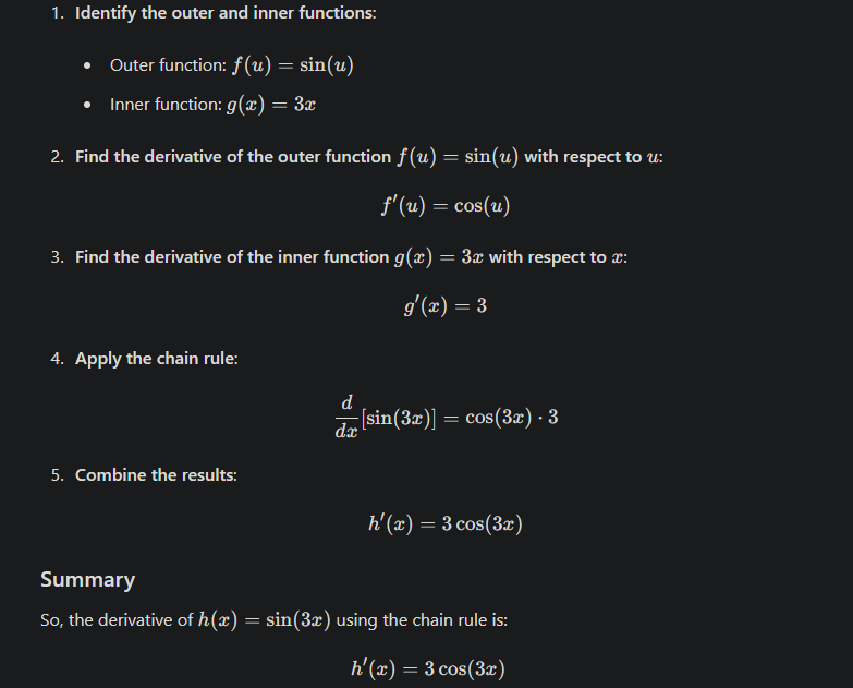
#chainrule

Probability - Law of Large Numbers

$(1/\sqrt{n})$

A probability function maps events onto real values ${P: \mathcal{A} \subseteq \mathcal{S} \rightarrow [0,1]}$. The probability, denoted $P(\mathcal{A})$, of an event $\mathcal{A}$ in the given sample space $\mathcal{S}$, has the following properties:

• The probability of any event $\mathcal{A}$ is a nonnegative real number, i.e., $P(\mathcal{A}) \geq 0$;
• The probability of the entire sample space is $1$, i.e., $P(\mathcal{S}) = 1$;
• For any countable sequence of events $\mathcal{A}1, \mathcal{A}_2, \ldots$ that are *mutually exclusive* (i.e., $\mathcal{A}_i \cap \mathcal{A}_j = \emptyset$ for all $i \neq j$), the probability that any of them happens is equal to the sum of their individual probabilities, i.e., $P(\bigcup{i=1}^{\infty} \mathcal{A}i) = \sum{i=1}^{\infty} P(\mathcal{A}_i)$.

  Random Variables

 random variables can be much coarser than the raw sample space. We can define a binary random variable like “greater than 0.5” even when the underlying sample space is infinite,

Exercise